Main Engine Performance

---

​

Marine Main Engine Performance – Methodology Guide

This document explains how the application evaluates a vessel’s main engine performance using shop trial references and monthly performance records.

---

​

1) Data sources we use

• Shop trial reference: For each vessel, we keep the reference curves (and equations) for the key parameters. These represent how the engine should behave at different loads when it was in reference condition.
• Monthly performance record: For each selected date, we fetch the vessel’s recorded operating data (engine load, pressures, temperatures, speeds, fuel data, etc.). These are the “as-sailed” measurements.

---

​

2) Parameters assessed

The dashboard reviews the following, plus a few combined/derived items:

• Fuel Index
• Engine Speed
• $P_{max}$
• $P_{comp}$
• Scavenge Pressure
• SFOC (Specific Fuel Oil Consumption)
• Turbocharger related items (per turbocharger): T/C speed, temperature before T/C, temperature after T/C
• Derived metrics: Pressure Rise ($P_{max} - P_{comp}$) and Torque Rich Index

---

​

3) How the reference is obtained

• For each parameter, we look up the vessel’s shop trial curve and read the expected value at the current engine load. Where the shop trial data must be converted into a reference curve, we generate a mathematical model.
• For turbocharger parameters that have multiple units on the same engine, we treat each index separately (e.g., “T/C Speed #1”, “T/C Speed #2”).

​

Generating a Reference Curve via Regression Analysis:

• To establish a reliable performance baseline from raw data, the discrete points from the shop trial report are used to generate a continuous mathematical model. This process, known as curve fitting or regression analysis, allows for the accurate estimation of any parameter at any given engine load. The following steps outline the procedure using the maximum combustion pressure ($P_{max}$) as an example.

---

​

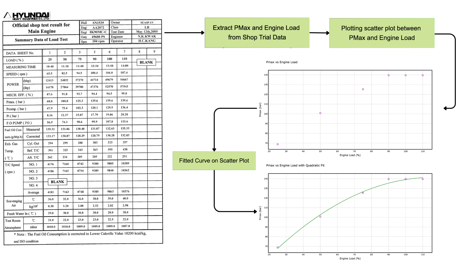
3.1) Data Extraction and Visualization

The initial step is to extract the independent variable (Engine Load, denoted as $x$) and the corresponding dependent variable (the parameter of interest, e.g., $P_{max}$, denoted as $y$) from the shop trial data. From the shop trial table for $P_{max}$:

• Engine Load ($x$): [25, 50, 75, 90, 100, 110] in %
• $P_{max}$ ($y$): [68.8, 100.8, 125.3, 139.6, 139.6, 139.6] in bar

These data points $(x_i, y_i)$ are then plotted on a scatter graph to visually inspect the underlying relationship.

---

​

3.2) Model Fitting and Validation

Given the known non-linear relationship between engine load and parameters like $P_{max}$, a polynomial regression model is an effective choice to represent the data. We fit the data to a polynomial function of an appropriate degree $n$: $y(x) = a_n x^n + a_{n-1} x^{n-1} + \dots + a_1 x + a_0$ The process involves calculating the coefficients ($a_n, \dots, a_0$) that create a curve passing as closely as possible to the data points. The quality of this fit is crucial. We quantify it using the Coefficient of Determination ($R^2$). For a model to be accepted as a reliable reference, we require an $R^2$ value greater than 0.95, ensuring it accurately represents the engine’s original performance characteristics.

---

​

3.3) Application of the Reference Model

With a validated mathematical model, you can now accurately estimate the expected performance parameter for any given engine load, not just the discrete points tested during the shop trial. By substituting the current engine load ($x_{current}$) into the derived equation, you obtain the expected reference value ($y_{reference}$). This reference is then compared against the currently measured value to assess the engine’s real-time operational efficiency and health.

---

​

4) Normalising Measured Values (ISO Correction)

To ensure a valid comparison between live operational data and the engine’s baseline shop trial performance, measured values must be adjusted to a common set of standard ambient conditions. This normalization process is governed by the ISO 3046-1 standard. The correction accounts for deviations in ambient conditions from the established reference points. The primary variables considered for this adjustment are:

• Charge Air Temperature ($T_{air}$)
• Charge Air Coolant Temperature ($T_{cw}$)
• Ambient Air Pressure ($p_a$)

​

Correction Model for Maximum Combustion Pressure ($P_{max}$)

The observed maximum combustion pressure ($P_{max, obs}$) is highly sensitive to the temperature of the charge air and its coolant. The correction formula adjusts the observed value based on how much these temperatures deviate from the ISO standard reference temperature ($T_{ref}$), which is 25 °C (298 K). The general scientific model for this correction is as follows: $P_{max, iso} = P_{max, obs} + \left[ K_{air}(T_{air} - T_{ref}) + K_{cw}(T_{cw} - T_{ref}) \right] \times (1 + P_{max, obs})$ Definition of Terms:

• $P_{max, iso}$ : The ISO-corrected maximum combustion pressure in bar. This is the value comparable to the shop trial reference.
• $P_{max, obs}$ : The observed (measured) maximum combustion pressure in bar.
• $T_{air}$ : The observed charge air inlet temperature in °C.
• $T_{cw}$ : The observed charge air coolant (water) inlet temperature in °C.
• $T_{ref}$ : The ISO standard reference temperature (25 °C).
• $K_{air}$ : The engine-specific correction factor for air temperature deviation.
• $K_{cw}$ : The engine-specific correction factor for coolant temperature deviation.

---

​

Example Application

Using the specific correction factors for a given engine:

• $K_{air} = 2.198 \times 10^{-3}$
• $K_{cw} = -0.81 \times 10^{-3}$

We can substitute these constants into the general model to derive the precise formula for the vessel: $P_{max, iso} = P_{max, obs} + \left[ (2.198 \times 10^{-3})(T_{air} - 25) - (0.81 \times 10^{-3})(T_{cw} - 25) \right] \times (1 + P_{max, obs})$ This equation isolates the engine’s performance from the influence of changing ambient temperatures, allowing for a true “like-for-like” comparison against its reference data.

---

​

5) Judging performance – deviation

For each parameter, we take the ISO corrected measured value (current condition) and the shop trial value (reference at the same load). We then compute the percentage difference between the two, which we call the deviation. The formula used is: $\text{Deviation} (\%) = \frac{\text{ISO Corrected Value} - \text{Shop Trial Value}}{\text{Shop Trial Value}} \times 100$

---

​

6) What is displayed on each card

Each parameter card shows:

• ISO corrected value (what the measurement would be under standard conditions)
• Measured value (what was recorded)
• Shop trial value (expected at the same load)
• Deviation and color classification
• A performance chart: reference curve, shop trial points, and the current measured point
• A trend chart of deviation over time, with range controls (6 months, 1 year, max, or custom)

---

​

7) Special/derived metrics

• Pressure Rise ($P_{max} - P_{comp}$): Calculated directly from $P_{max}$ and $P_{comp}$ in the same record and compared with a reference curve for pressure rise.
• Torque Rich Index: Compares the current load implied by engine speed with the expected shop trial load at that speed. If a vessel‑specific load‑from‑speed curve is provided in shop trial data, that is used. Otherwise a fallback curve is used and a warning is logged. The index itself is treated like a deviation; values near zero are normal.
• SFOC (Corrected): Uses the record’s fuel and power information to derive measured SFOC. If the record also contains an already-corrected SFOC value, that is preferred for judging against the reference curve.

---

​

8) Turbocharger handling

If the vessel has multiple turbochargers, the app creates separate cards per unit (e.g., “T/C Speed #1”, “T/C Speed #2”). Each unit:

• Uses its own measured value
• Uses the correct reference curve
• Gets its own color classification and trend history

---

​

9) AI Insights

For each parameter on a given vessel and date, a short “AI Insight” is generated to give quick, action‑oriented context (e.g., “consistent with low load” or “monitor fouling risk”).

---

​

10) Data ranges and trend history

The trend chart lets you view deviation over configurable time ranges (6 months, 1 year, maximum history, or custom start/end). The values shown are the same deviation percentages described above, allowing you to spot patterns or gradual drift.

---

​

11) Interpretation guidance

• Negative deviation for some parameters can be acceptable, depending on context (e.g., slightly lower engine speed can indicate the engine is running light). The insights and color rules help you prioritise.
• Consider multiple parameters together. For example, low scavenge pressure with low T/C speed and rising exhaust temperatures points to air‑side issues.
• Be cautious when judging very low engine loads; several parameters naturally behave differently, and trend context becomes important.

---

​

12) What to do with reds and yellows

• Red: Plan checks and remedial actions. Look for corroborating parameters and recent trend direction. If persistent, schedule maintenance.
• Yellow: Monitor. If trending worse, schedule closer observation or cleaning tasks (e.g., air coolers, turbocharger checks) at the next convenient opportunity.

---

​

13) Summary

1. Normalize current measurements to standard conditions.
2. Compare them against the vessel’s own shop trial references at the same load.
3. Classify the gap using clear, fixed thresholds and display both the one‑off point and the history.
4. Provide short, contextual insights and store them once per vessel/date/parameter so the view is fast and consistent.

This approach aligns day‑to‑day operating observation with the vessel’s original baseline, helping crews and superintendents focus on what matters and plan maintenance with confidence.

---

​

Illustrated example: SFOC (Corrected)

What you are looking at in the card above:

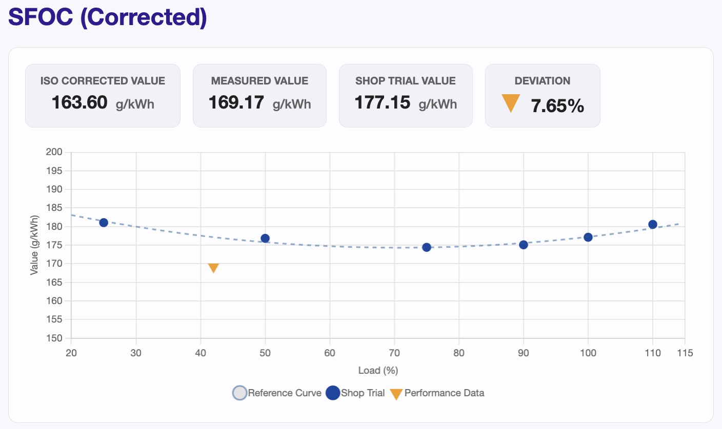
• Title: the parameter being assessed.
• Four tiles at the top:
  • ISO Corrected Value: today’s measurement normalised to standard ambient conditions.
  • Measured Value: the raw value in the monthly record.
  • Shop Trial Value: the expected value at the same load from the vessel’s reference curve.
  • Deviation: the percentage gap between today’s ISO corrected value and the shop trial value. A downward arrow means the value is below reference; an upward arrow means above reference.
• The chart:
  • Dotted curve: the reference shape across the full load range.
  • Blue dots: shop trial points.
  • Orange triangle: today’s point.

​

Deviation Calculation

The deviation is computed using the values shown in the figure.

• ISO Corrected Value = 163.60 g/kWh
• Shop Trial Value = 177.15 g/kWh

Using the formula: $\text{Deviation} (\%) = \frac{163.60 - 177.15}{177.15} \times 100 \approx -7.65\%$ This is displayed as 7.65% with a downward arrow to indicate it is below the reference. For SFOC, a lower value can be positive; always consider the wider context and trend.

---

​

Color coding and actions (applies to all cards and trends)

Color	Deviation band	What it means	Suggested action
Green	within $\pm5\%$	In line with reference	Continue normal operation; keep monitoring via trend.
Yellow	>$\pm5\%$ and $\le\pm10\%$	Noticeable difference	Review together with other parameters; plan checks at next convenient opportunity.
Red	>$\pm10\%$	Significant difference	Prioritise investigation; plan corrective action and monitor trend closely.

Note: The direction of deviation matters. For example, lower SFOC or slightly lower engine speed can be acceptable or even positive. The short insight next to each card provides context.

---

​

How to read the trend chart

• A stable line near zero means the parameter behaves like the reference over time.
• A slowly rising line shows gradual drift away from reference; combine with the card’s color to prioritise.
• Sudden spikes can be operational events; look for persistence across dates before drawing conclusions.